| LIBROW | ® |
| Products | Solutions | Vehicles | Articles | Inquiry | Contacts | My account |
Article 9
Gaussian filter, or Gaussian blur
Category. Digital signal and image processing (DSP and DIP) software development.
Abstract. The article is a practical tutorial for Gaussian filter, or Gaussian blur understanding and implementation of its separable version. Article contains theory, C++ source code, programming instructions and a sample application.
Limited offer
Professional Librow Calculatorvisit
for free
- Bessel functions
- gamma function
- complex numbers
7.4 MB for Windows
 |
Download Gaussian filter, or Gaussian blur for Win32 (zip, 890 kB) |
 |
Download Gaussian filter, or Gaussian blur C++ source code (zip, 4 kB) |

1. Introduction to Gaussian filter, or Gaussian blur
Gaussian filter is windowed filter of linear class, by its nature is weighted mean. Named after famous scientist Carl Gauss because weights in the filter calculated according to Gaussian distribution — the function Carl used in his works. Another name for this filter is Gaussian blur.
To get acquainted with filter window idea in signal and image processing read our “Filter window, or filter mask” article.
2. Understanding Gaussian filter, or Gaussian blur
First of all let us have a look at what that Gaussian distribution is. Gaussian distribution, or normal distribution, is really a function of probability theory. Often this function is referenced as bell-function because of its shape. The most general function formula is:
 |
(1) |
And its plot is depicted below — fig. 1.
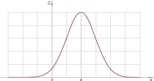 Fig. 1. Gaussian or normal distribution.
In our case we can suppose parameter a — which called distribution mean or statistical expectation — responsible for distribution shifting along x axis to be zero: a=0; and work with simplified form:
 |
(2) |
Thus the function is negative exponential one of squared argument. Argument divider σ plays the role of scale factor. σ parameter has special name: standard deviation, and its square σ2 — variance. Premultiplier in front of the exponent is selected the area below plot to be 1. Pay attention the function is defined everywhere on real axis x∈(−∞, ∞) which means it spreads endlessly to the left and to the right.
Now, first point is we are working in discrete realm, so our Gaussian distribution turns into the set of values at discrete points.
Second, we cannot work with something that spreads endlessly to the left and to the right. It means Gaussian distribution is to be truncated. The question is — where? Usually in practice used the rule of 3σ that is the part of Gaussian distribution utilized is x∈[−3σ, 3σ] — see fig. 2.
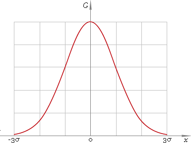 Fig. 2. Gaussian distribution truncated at points ±3σ.
Why? Good question. To understand that let us see how much we have trimmed. The area below truncated part is:
 |
(3) |
Now we can start up MatLab and type lines like:
G=inline('1/sqrt(2*pi)*exp(-x.^2/2)');
quad(G, -3, 3)
Which tells MatLab to calculate our integral (3). The result is
ans =
    0.9973
So, the area below our trimmed part is ≈0.997 — that is function is trimmed at points where we have accuracy better than 0.5%. Very good in our case.
Back to our discrete normal distribution: we are interested in points {x−N, x−N+1, ... , x−1, x0, x1, ... , xN−1, xN}, where x−n=−xn and xN=3σ, and respectively in values of normal distribution at these points: {G(x−N), G(x−N+1), ... , G(x−1), G(x0), G(x1), ... , G(xN−1), G(xN)}. So, we have 2N+1 value set {Gn | n=−N, −N+1, ... , N} where Gn=G(xn).
What shall we do now with this set of values? Use it as window weights! That means we have weighted window of 2N+1 size. To be perfect we are to scale our Gn: G'n=Gn/k so that ∑G'n=1 — sum of all of them to be one: G'n=Gn/∑Gn — which means k=∑Gn.
Thus, we have our window weights {G'n | n=−N, −N+1, ... , N} where G'n=Gn/k, Gn=G(xn), k=∑Gn and xN=3σ which means as well xn=3σn/N. To get expression for G'n for practical use let us write down the detailed formula:
 |
(4) |
As you can see we have simplification: σ is eliminated from consideration and G'n could be calculated easier via new values G"n and their sum k'.
How to use these weights? If we have some input signal S={si} then for every signal element si the new modified value s'i will be s'i=∑G'nsi+n, n=−N, −N+1, ... , N. In words that means “for every element put our window so that this element is in the center of the window, multiply every element in the window by corresponding weight and sum up all those products, the sum got is the new filtered value”.
Now we can write down step-by-step instructions for processing by 1D Gaussian filter or blur.
1D Gaussian filter, or Gaussian blur algorithm:
- Given window size 2N+1 calculate support points xn=3n/N, n=−N, −N+1, ... , N;
- Calculate values G"n;
- Calculate scale factor k'=∑G"n;
- Calculate window weights G'n=G"n/k';
- For every signal element:
- Place window over it;
- Pick up elements;
- Multiply elements by corresponding window weights;
- Sum up products — this sum is the new filtered value.
Let us proceed with 2D case.
3. 2D case
Expression for 2D Gaussian distribution is:
 |
(5) |
And its plot is depicted below — fig. 3.
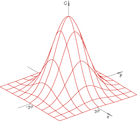 Fig. 3. 2D Gaussian or normal distribution.
Gaussian distribution has surprising property. Look, its expression could be rewritten as:
 |
(6) |
Which means 2D distribution is split into a pair of 1D ones, and so, 2D filter window (fig. 3) is separated into a couple of 1D ones from fig. 2. Filter version that utilizes this fact is called separable one.
In practice it means that to apply filter to an image it is enough to filter it in horizontal direction with 1D filter and then filter the result with the same filter in vertical direction. Which direction first really makes no difference — our operation is commutative. Thus,
2D separable Gaussian filter, or Gaussian blur, algorithm:
- Calculate 1D window weights G'n;
- Filter every image line as 1D signal;
- Filter every filtered image column as 1D signal.
2D Gaussian filtering with [2N+1]×[2N+1] window is reduced to a couple of 1D filterings with 2N+1 window. That means significant speed-up especially for large images because of jump from O(N2) to O(N) number of operations.
Now, when we have the algorithm, it is time to write some code — let us come down to programming.
4. 2D Gaussian filter, or 2D Gaussian blur programming
We are starting with 2D filter because 1D one could be easily got just by treating signal as one-line image and canceling vertical filtering.
First of all a couple of simple auxiliary structures.
//   Internal auxiliary structure - data array size descriptor
struct CSize
{
   unsigned int x;   //   Array width
   unsigned int y;   //   Array height

   //   Default constructor
   CSize(): x(0), y(0) {}
   //   Constructor with initialization
   CSize(unsigned int _x, unsigned int _y): x(_x), y(_y) {}

   //   Initialization
   void Set(unsigned int _x, unsigned int _y) { x = _x; y = _y; }
   //   Area
   unsigned int Area() const { return x * y; }
};

//   Internal auxiliary structure - array descriptor
struct CArray
{
   CSize Size;   //   Array size
   T *Buffer;    //   Element buffer

   //   Default constructor
   CArray(): Buffer(NULL) {}
   //   Constructors with initialization
   CArray(T *_Buffer, const CSize &_Size): Buffer(_Buffer), Size(_Size) {}
   CArray(T *_Buffer, unsigned int _N): Buffer(_Buffer), Size(_N, 1) {}
};
CSize structure keeps the image size and CArray structure is image descriptor — its size and pointer to image data. Now more complicated structure —
our Gaussian window.
//   Internal auxiliary structure - filter window descriptor
struct CWindow
{
   double *Weights;   //   Window weights
   unsigned int Size;   //   Window size

   //   Default constructor
   CWindow(): Weights(NULL), Size(0), Correction(.5 - double(T(.5))) {}
   //   Destructor
   ~CWindow() { if (Weights) delete[] Weights; }

   //   Filter window creation
   bool Create(unsigned int _Size);

   //   FILTER WINDOW APPLICATION
   //     _Element - start element in signal/image
   T Apply(const T *_Element) const
   {
      //   Apply filter - calculate weighted mean
      double Sum = 0.;
      const double *WeightIter = Weights;
      const T *ElIter = _Element;
      const double *const End = Weights + Size;
      while (WeightIter < End)
         Sum += *(WeightIter++) * double(*(ElIter++));
      return T(Sum + Correction);
   }

protected:
   const double Correction;   //   Result correction
};
CWindow structure designed to keep window size and set of weights, as well it has two methods to calculate weights and to apply 1D Gaussian filter starting from
a given image element: Create and Apply. As you can see Apply code is trivial and code for Create is a little bit more complicated:
//   FILTER WINDOW CREATION
//     _Size - window size
template <class T> bool TGaussianBlur<T>::CWindow::Create(unsigned int _Size)
{
   //   Allocate window buffer
   Weights = new double[_Size];
   //   Check allocation
   if (!Weights)
      //   Window buffer allocation failed
      return false;
   //   Set window size
   Size = _Size;
   //   Window half
   const unsigned int Half = Size >> 1;
   //   Central weight
   Weights[Half] = 1.;
   //   The rest of weights
   for (unsigned int Weight = 1; Weight < Half + 1; ++Weight)
   {
      //   Support point
      const double x = 3.* double(Weight) / double(Half);
      //   Corresponding symmetric weights
      Weights[Half - Weight] = Weights[Half + Weight] = exp(-x * x / 2.);
   }
   //   Weight sum
   double k = 0.;
   for (unsigned int Weight = 0; Weight < Size; ++Weight)
      k += Weights[Weight];
   //   Weight scaling
   for (unsigned int Weight = 0; Weight < Size; ++Weight)
      Weights[Weight] /= k;
   //   Succeeded
   return true;
}
The method implements steps 1–4 of 1D Gaussian filter algorithm to calculate weights according to expression (4) and utilizes window symmetry G−n=Gn.
Now, the last problem to be solved before we can start filtering the image is its extension.
5. Extension
There is a problem every windowed filter deals with. Being placed at the edge filter window lacks for data elements to be processed. There are two ways to solve the problem: first is not to process edges and second, cleverer one, to extend data across edges. We are taking the second approach and extending our data like depicted in fig. 4.
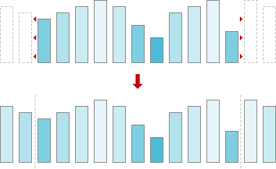 Fig. 4. Data extension.
And here is CExtension class that will do that job for us.
//   Internal auxiliary structure - array extension descriptor
struct CExtension: public CArray
{
   unsigned int Margin;   //   Extension margins

   enum EMode {ModeHorizontal, ModeVertical};

   //   Default cosntructor
   CExtension(): Margin(0), Mode(ModeHorizontal) {}
   //   Destructor
   ~CExtension() { if (Buffer) delete[] Buffer; }

   //   Mode setting
   void SetMode(EMode _Mode) { Mode = _Mode; }
   //   Extension memory allocation
   bool Allocate(unsigned int _N, unsigned int _W)
   { return _Allocate(CSize(_N, 1), _W >> 1); }
   bool Allocate(const CSize &_Size, unsigned int _W)
   { return _Allocate(_Size, _W >> 1); }
   //   Pasting data into extension from data array
   void Paste(const T * _Start);
   //   Extension
   void Extend();

protected:
   EMode Mode;   //   Current mode

   //   Extension memory allocation
   bool _Allocate(const CSize &_Size, unsigned int _Margin);
};
The job is done inside methods _Allocate, Paste and Extend. _Allocate method allocates space in memory enough to keep
extended image line or column.
//   EXTENSION MEMORY ALLOCATION
//     _Size   - signal/image size
//     _Margin - extension margins
template <class T> bool TGaussianBlur<T>::CExtension::_Allocate(
   const CSize &_Size, unsigned int _Margin)
{
   //   Allocate extension buffer
   Buffer = new T[(_Size.x > _Size.y ? _Size.x : _Size.y) + (_Margin << 1)];
   //   Check buffer allocation
   if (!Buffer)
      //   Buffer allocation failed
      return false;
   //   Initialize size descriptors
   Size = _Size;
   Margin = _Margin;
   //   Succeeded
   return true;
}
Method Paste inserts image line or column at proper place in extension.
//   PASTING DATA LINE/COLUMN INTO EXTENSION FROM DATA ARRAY
//     _Start - start postion in image/signal to paste from
template <class T> void TGaussianBlur<T>::CExtension::Paste(const T *const _Start)
{
   if (Mode == ModeHorizontal)
   {
      //   Paste line
      memcpy(Buffer + Margin, _Start, Size.x * sizeof(T));
   }
   else
   {
      //   Stop position
      const T *const Stop = _Start + Size.Area();
      //   Array iterator
      const T *ArrIter = _Start;
      //   Extension iterator
      T *ExtIter = Buffer + Margin;
      //   Paste array column element by element
      while (ArrIter < Stop)
      {
         //   Copy line
         *(ExtIter++) = *ArrIter;
         //   Jump to the next line
         ArrIter += Size.x;
      }
   }
}
Pasting has two modes — horizontal and vertical. In horizontal mode line is copied into the extension and in vertical mode column is copied element by element.
Method Extend mirrors pasted data.
//   EXTENSION CREATION
template <class T> void TGaussianBlur<T>::CExtension::Extend()
{
   //   Line size
   const unsigned int Line = Mode == ModeHorizontal ? Size.x : Size.y;
   //   Stop position
   const T *const Stop = Buffer - 1;
   //   Left extension iterator
   T *ExtLeft = Buffer + Margin - 1;
   //   Left array iterator
   const T *ArrLeft = ExtLeft + 2;
   //   Right extension iterator
   T *ExtRight = ExtLeft + Line + 1;
   //   Left array iterator
   const T *ArrRight = ExtRight - 2;
   //   Create extension line element by element
   while (ExtLeft > Stop)
   {
      //   Left extension
      *(ExtLeft--) = *(ArrLeft++);
      //   Right extension
      *(ExtRight++) = *(ArrRight--);
   }
}
Now we have everything to program filtering method.
//   2D GAUSSIAN BLUR
//     pImage  - input image
//     pResult - output image, NULL for inplace processing
//     N       - width of the image
//     M       - height of the image
//     W       - window size
template <class T> bool TGaussianBlur<T>::Filter(T *pImage, T *pResult,
   unsigned int N, unsigned int M, unsigned int W) const
{
   //   Check input data consistency
   if (!Consistent(pImage, CSize(N, M), W))
     return false;
   //   Allocate extension
   CExtension Extension;
   if (!Extension.Allocate(CSize(N, M), W))
      return false;
   //   Create image descriptor
   CArray Image(pImage, CSize(N, M));
   //   Create filter window
   CWindow Window;
   if (!Window.Create(W))
      return false;
   //   Stop postion
   const T * ExtStop = Extension.Buffer + Extension.Size.x;
   //   Result iterator
   T *ResIter = pResult ? pResult : pImage;
   //   Image iterator
   const T *ImIter = Image.Buffer;
   //   Image stop position
   const T * ImStop = Image.Buffer + Image.Size.Area();
   //   Filter line by line
   while (ImIter < ImStop)
   {
      //   Paste image line into extension
      Extension.Paste(ImIter);
      //   Extend image line
      Extension.Extend();
      //   Extension iterator
      const T *ExtIter = Extension.Buffer;
      //   Apply filter to every pixel of the line
      while (ExtIter < ExtStop)
         *(ResIter++) = Window.Apply(ExtIter++);
         //   Move to the next line
      ImIter += Image.Size.x;
   }
   //   Initialize image descriptor with filter result
   Image.Buffer = pResult ? pResult : pImage;
   //   Set vertical extension mode
   Extension.SetMode(CExtension::ModeVertical);
   //   Extension stop position
   ExtStop = Extension.Buffer + Extension.Size.y;
   //   Result column iterator
   T *ResColumnIter = pResult ? pResult : pImage;
   //   Image iterator
   ImIter = Image.Buffer;
   //   Image stop position
   ImStop = Image.Buffer + Image.Size.x;
   //   Filter column by column
   while (ImIter < ImStop)
   {
      //   Paste image column into extension
      Extension.Paste(ImIter++);
      //   Extend image column
      Extension.Extend();
      //   Extension iterator
      const T *ExtIter = Extension.Buffer;
      //   Result pixel iterator
      ResIter = ResColumnIter;
      //   Apply fitler to every pixel of the column
      while (ExtIter < ExtStop)
      {
         *ResIter = Window.Apply(ExtIter++);
         ResIter += Image.Size.x;
      }
      //   Move to the next column
      ++ResColumnIter;
   }
   //   Succeeded
   return true;
}
Structure of the method is quite straightforward: input parameters check, memory allocation, window weights calculation, applying 1D filter in horizontal direction (first loop) and applying it in vertical direction (second loop). Parameters check is a short function below.
//   Internal auxiliary functions - check input data consistency
bool Consistent(const T *_Image, const CSize &_Size, unsigned int _W) const
{
   return  _Image && _Size.x && _Size.y && _W &&
      _Size.x > (_W >> 1) && _Size.y > (_W >> 1) && _W & 1;
}
Which means pointer to image should not be NULL, image and filter window sizes should be some positive numbers, window size 2N+1≡_W
should be odd number and N should be less than image size in any direction.
6. 1D Gaussian filter, or Gaussian blur programming
1D filter is truncated version of 2D filter:
//   1D GAUSSIAN BLUR
//     pSignal - input signal;
//     pResult - output signal, NULL for inplace processing
//     N       - length of the signal
//     W       - window size, odd positive number
template <class T> bool TGaussianBlur<T>::Filter(T *pSignal, T *pResult,
   unsigned int N, unsigned int W) const
{
   //   Check input data cosnsitency
   if (!Consistent(pSignal, N, W))
      return false;
   //   Allocate extension
   CExtension Extension;
   if (!Extension.Allocate(N, W))
      return false;
   //   Create signal descriptor
   const CArray Signal(pSignal, N);
   //   Paste signal into extension
   Extension.Paste(Signal.Buffer);
   //   Extend signal
   Extension.Extend();
   //   Create filter window
   CWindow Window;
   if (!Window.Create(W))
      return false;
   //   Extension iterator
   const T *ExtIter = Extension.Buffer;
   //   Extension stop position
   const T *const ExtStop = Extension.Buffer + Extension.Size.x;
   //   Result iterator
   T *ResIter = pResult ? pResult : pSignal;
   //   Filter - apply to every element
   while (ExtIter < ExtStop)
      *(ResIter++) = Window.Apply(ExtIter++);
   //   Succeeded
   return true;
}
You can see familiar steps here just now filter makes one pass along signal array.
Our separable Gaussian filter library is ready! You can download full source code here:
 |
Download Gaussian filter, or Gaussian blur C++ source code (zip, 4 kB) |
Full file listings are available online as well:
- Appendix A.1. Gaussian filter, or Gaussian blur source code — gaussianblur.h — file of declarations;
- Appendix A.2. Gaussian filter, or Gaussian blur source code — gaussianblur.cpp — file of implementation.
6. How to use
Pay attention that our solution is universal. First, our filter has window of arbitrary size. Second, we have developed class template that suits any type of input data —
TGaussianBlur<unsigned char> BlurFilter;TGaussianBlur<short> BlurFilter;TGaussianBlur<float> BlurFilter;TGaussianBlur<int> BlurFilter;TGaussianBlur<unsigned int> BlurFilter;— all these declarations are valid and will process your data graciously.
To use the filter you should include header file gaussianblur.h and place in your code lines like:
...Usually at the top of the file
//   Include Gaussian blur header
#include "gaussianblur.h"
.
...Some code here
.
   ...Inside your signal/image processing function
   //   Create instance of Gaussian blur filter
   TGaussianBlur<double> BlurFilter;
   //   Apply Gaussian blur
   BlurFilter.Filter(pImage, NULL, 512, 512, 13);
Here image is stored as double array of 512×512 size and it is filtered in-place with Gaussian window of 13×13 pixels width.
And now — an application to play around!
7. Color Gaussian blur
 |
Download Gaussian filter, or Gaussian blur for Win32 (zip, 890 kB) |
We have created an application to see Gaussian filter in action. The sample package includes 3 files — the applications, sample image and description:
- gaussianblur.exe — Gaussian filter,
- sample.bmp — 24-bit sample image,
- readme.txt — description.
Be aware of the fact, that this sample uses OpenGL, so it should be supported by your system (usually that is the case).
8. How to use
Start up gaussianblur.exe application. Load the image.
 Fig. 5. Original image.
Set filter window size: Set >> Window size... or click w-button in toolbar, in dialog key in size, for instance 13. Blur image with Gaussian filter by choosing Set >> Filter or clicking F-button in toolbar. See the result.
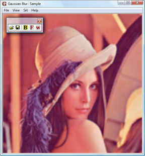 Fig. 6. Image blurred by Gaussian filter.
|
|
|||||||||||||
|
|||||||||||||


